Date: 10/6/2016
Author: Descreye Solutions
A histogramic distribution is the term used for a distribution whose characteristics are defined by intervals of percentiles obtained from raw data. The percentiles become the bounds for a series of uniform distributions that are sampled from to obtain a random variate. Two random numbers are needed to generate a random variate from the histogramic distribution. The first sample determines which uniform distribution to use from the series of uniform distributions. The second sample is a random number sample from the uniform distribution between the bounds of the previously selected uniform distribution. The number of uniform distributions is unimportant to be a histogramic distribution. The number of distributions can be denoted by hyphenating the amount after histogramic when describing the distribution (i.e. histogramic-6 distribution).
If the following data denoted 10 observations from a process:
| Observation | Value |
| 1 | 10.1 |
| 2 | 8.2 |
| 3 | 9.5 |
| 4 | 12.0 |
| 5 | 11.8 |
| 6 | 10.2 |
| 7 | 15.1 |
| 8 | 9.0 |
| 9 | 25.7 |
| 10 | 10.8 |
To produce a histogramic-6 distribution, percentiles are identified at intervals of 1/(n-1), if n is the hyphenated number, from 0 to 1. So in this case the interval is 1/(6-1) which equals .2. So the following shows the table of percentile values of the data.
| Percentile | Value |
| 0 | 8.2 |
| .2 | 9.4 |
| .4 | 10.2 |
| .6 | 11.2 |
| .8 | 12.6 |
| 1 | 25.7 |
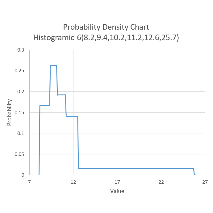
Given this information our distribution could be completely defined using the shorthand "histogramic-6(8.2,9.4,10.2,11.2,12.6,25.7)". This should be interpreted that the data will be sampled from a series of 5, (n-1), uniform distributions with the bounds defined in parenthesis. So 20% of the data will be between 8.2 and 9.4, 20% will be between 9.4 and 10.2, and so on. A graph of the probability distribution is shown below.
The distribution can then be sampled by sampling a random number from the discrete uniform distribution between 0 and (n-1). In this case that is uniform(0,5). If our random number was 2 we would then sample a random number from the continuous uniform distribution between the bounds of the second and third values in the distribution shorthand. In this case, with a random number of 2, we would sample from uniform(9.4,10.2). This would then give us a random variate that is representative of the histogramic distribution.
OPS uses the histogramic-6 distribution to automatically fit raw observation data into a random number generating distribution. Although a histogramic distribution is almost certainly not an exact replication of the real life randomness, it can be an accurate estimate for quick modeling. The benefit of the histogramic distribution is that it can mimic any single-mode distribution, and, as such, makes it unnecessary for a user to define the distribution. This makes it extremely easy to create a simulation in OPS if there is existing data.